Anatomy of the Mandelbrot set

The Mandelbrot set defined as a subset of the complex plane, the calculation that decides membership, and the shapes and dimension of its boundary.

13 minutes read

2726 words

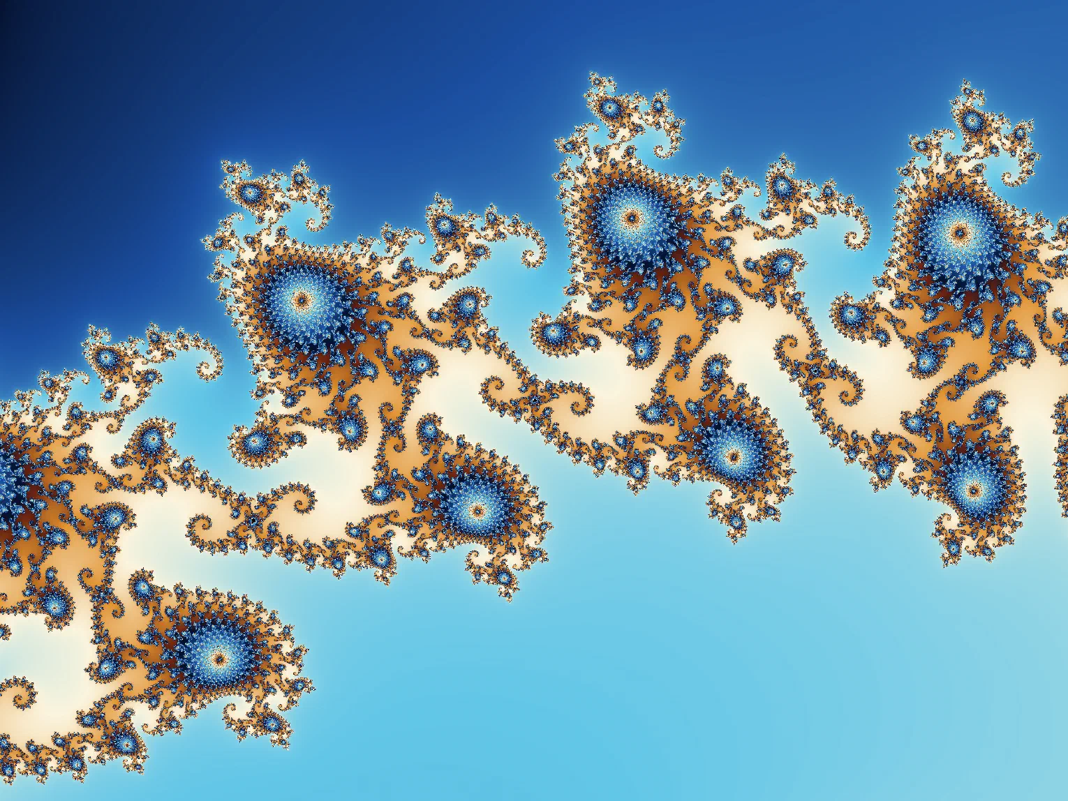
The pictures that carry the name Mandelbrot show a black bulb with spirals and curls along its edge. They are coloured in bands, and magnifying the edge reveals more detail without end. Those pictures are portraits of a set of complex numbers. One short calculation, repeated, decides which numbers belong. This page defines the set, works that calculation, and names the shapes the picture turns out to hold.

Assumed knowledge

Complex numbers, and the notation for writing a set and its members. Both are built up in numbers and sets .

Polar form, which names a point of the plane by a distance and an angle. It is built up in angles and polar form .

Iteration, which is applying one rule to its own output over and over, together with the words orbit, bounded and fixed point. That is iteration and orbits .

Nothing else. The test that decides membership is one line of arithmetic, repeated.

Ground covered

The Mandelbrot set defined as a subset of the complex numbers, and the orbit that decides which numbers belong. Why that orbit starts at zero. Squaring read as a rotation of the plane. The escape radius, which turns a test over infinitely many steps into a finite one. The two components whose boundaries are known in closed form, the dimension of the boundary, and the quantity that is still open.

Subset of the complex plane

Each complex number is drawn as a point, with its real part measured along the horizontal axis and its imaginary part up the vertical one. The set of all of them is written $\mathbb{C}$ .

The Mandelbrot set, written $M$ , is a subset of $\mathbb{C}$ . Every point of the plane is either a member of it or not, and one calculation settles which. That calculation is the subject of the next section.

The set is bounded. Every member lies within distance 2 of the origin, which the section on the escape radius proves. The whole of $M$ therefore fits in a small part of the plane.

Membership is not decided by nearness. Two values of $c$ a millionth apart can fall on opposite sides, and that is why the boundary carries detail at every magnification. The picture at the top of this page is one small piece of that boundary.

Orbit of zero

Fix a complex number $c$ . Apply the map $z \mapsto z^2 + c$ over and over, starting from zero. The map is called quadratic, because $z$ appears squared and no higher power of it appears.

The name describes the rule that is repeated, rather than the result of repeating it. Applying the rule twice gives $z^4 + 2cz^2 + c^2 + c$ , where $z$ now reaches the fourth power. Applying it $n$ times reaches the power $2^n$ , so ten steps reach 1024. The rule stays quadratic however often it runs. Squaring and adding are the ordinary arithmetic of complex numbers. The result is a sequence.

That sequence is the orbit of zero, which is the orbit of the map from the starting point 0. Three worked examples, each computed by squaring and adding:

$c = -1$

the orbit runs $0,\; -1,\; 0,\; -1,\; 0$ and repeats forever.

$c = i$

the orbit runs $0,\; i,\; -1+i,\; -i,\; -1+i,\; -i$ and repeats after the first two terms.

$c = 1$

the orbit runs $0,\; 1,\; 2,\; 5,\; 26,\; 677$ and grows without limit.

The first two orbits above stay bounded, which means one fixed distance from the origin holds every term. The third escapes, which means its moduli grow without limit. The Mandelbrot set $M$ is the set of values of $c$ whose orbit of zero stays bounded.¹

So $-1$ and $i$ belong to $M$ . The value $1$ escapes, and lies outside it. The figure above marks each of those, with a fourth value that also escapes.

Here $\mathbb{C}$ is the set of all complex numbers, and $R$ is one distance that holds every term of the orbit inside it. Which distance does not matter, only that one exists.

The starting value is zero for a reason. The derivative of a map at a point says how much it stretches a small step taken from there. That stretch is the test separating an attracting fixed point from a repelling one. For $f_c(z) = z^2 + c$ the derivative is $2z$ , so at zero it stretches nothing. A point where the derivative is zero is a critical point. The orbit of the critical point decides the behaviour of every other orbit. One sequence per value of $c$ is therefore enough.¹

The two letters carry different roles. The variable $z$ moves along the sequence. The variable $c$ is fixed for the whole sequence, and the picture is drawn over $c$ . A point of the image is a value of $c$ , never a value of $z$ .

Squaring as rotation

Write $r$ for the modulus of $z$ , which is its distance from the origin, and $\theta$ for its argument, which is its direction. Polar form then gives $z = r e^{i\theta}$ .

Multiplying two complex numbers multiplies their moduli and adds their arguments. Setting both factors to $z$ in that rule gives the geometric content of the map.

Squaring doubles the argument and squares the modulus. One step of equation (1) is three operations in sequence:

1. Rotate the point to twice its angle.
2. Scale its distance to the square of itself.
3. Translate it by $c$ .

The unit circle is the set of points at modulus one, and squaring behaves differently on each side of it. A point with $r < 1$ has $r^2 < r$ and moves inward. A point with $r > 1$ has $r^2 > r$ and moves outward. Under repeated squaring alone, with $c = 0$ , every point inside the unit circle converges to the origin. Every point outside it escapes. The circle itself is preserved.

Adding $c$ breaks that separation. A point moved inward by squaring can be moved back outside by the translation. The two operations together produce the boundary shown below.

Escape radius

Once the modulus of a term passes two, the orbit escapes. The bound follows from the reverse triangle inequality, which states that $|x + y| \ge |x| - |y|$ for any two complex numbers. Suppose $|z_n| > 2$ and $|z_n| \ge |c|$ . Then

The second line applies the inequality. The third uses $|c| \le |z_n|$ . Write $\lambda = |z_n| - 1$ . The factor $\lambda$ exceeds one, because $|z_n| > 2$ . So $|z_{n+1}| \ge \lambda |z_n| > |z_n|$ . The modulus grows, and $\lambda$ grows with it. After $k$ further steps $|z_{n+k}| \ge \lambda^k |z_n|$ , and that bound grows without limit.

The condition $|z_n| \ge |c|$ costs nothing. If $|c| > 2$ then $z_1 = c$ already has modulus above two, so such a $c$ lies outside $M$ . Every $c$ that needs testing satisfies $|c| \le 2$ . Every term under test satisfies $|z_n| > 2 \ge |c|$ . The whole set lies inside the disc of radius two, and one comparison decides escape.¹

def escapes(c, nmax=400):
    """Return the step at which the orbit of 0 leaves the disc of radius 2."""
    z = 0j
    for n in range(nmax):
        z = z * z + c
        if abs(z) > 2.0:
            return n
    return None

A returned value of None means the orbit survived nmax steps. That is evidence of membership, never proof. No finite computation decides membership for a point of the boundary.

Two exact shapes

The interior of $M$ breaks into components. A component is one connected piece of that interior, a region that holds together and touches no other such region. Two of them have shapes given in closed form, and both are drawn over the computed set below.

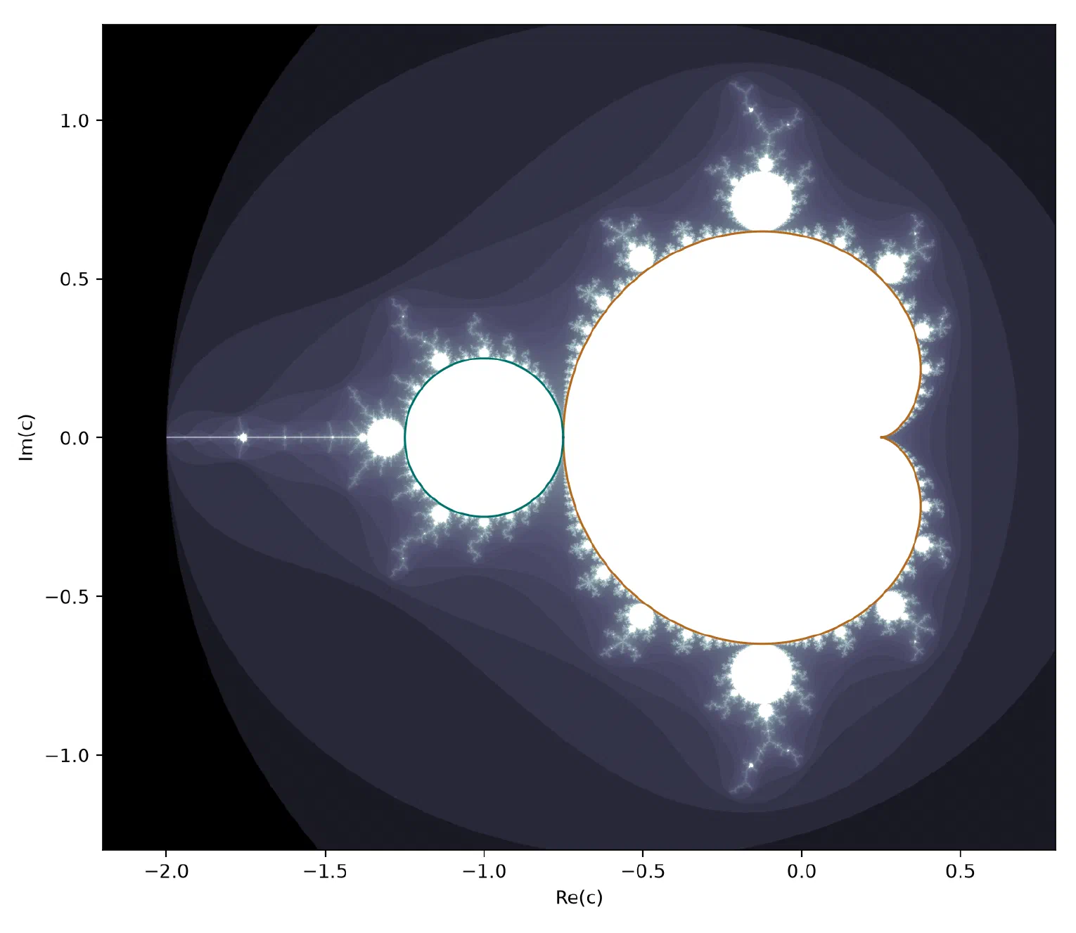
The main cardioid is the largest component, the heart-shaped region on the right of the figure. It holds the values of $c$ for which $f_c$ has an attracting fixed point. A fixed point is a value $z$ that the map leaves where it is, so $z = z^2 + c$ . It attracts when nearby points move towards it under repeated application. That happens when the derivative there has modulus below one, which is $|2z| < 1$ .

Substitute $\mu = 2z$ . Then $z = \mu/2$ , and the fixed-point equation rearranges to $c = z - z^2$ . Therefore

and the condition $|2z| < 1$ becomes $|\mu| < 1$ . The main cardioid is the image of the open unit disc under equation (5).¹ Its boundary follows from $\mu = e^{i\theta}$ ,

The component attached at $c = -3/4$ holds values of $c$ with an attracting orbit of period two. An orbit has period two when it returns to its starting value after two steps. The orbit for $c = -1$ does that. That component is a disc of radius one quarter centred at $-1$ .¹ The circle in the figure is that disc drawn from its formula. Components of higher period surround the cardioid.

Filaments and islands

Adrien Douady and John Hubbard proved in 1985 that $M$ is connected, meaning it forms a single piece. They built a conformal isomorphism.¹ It runs between the outside of $M$ and the outside of the closed unit disc. A conformal isomorphism is a map between two regions. It preserves angles, and a map of the same kind undoes it. Its existence shows the outside of $M$ is as simple as the outside of a disc.

Every island in a rendering is therefore joined to the main body by a filament. That includes the small copies along the horizontal axis. A filament can be thinner than the pixel grid, so the islands look separate.

Shishikura’s theorem

The boundary of $M$ is the set of points that have both members of $M$ and non-members arbitrarily close by. Its Hausdorff dimension is two. Hausdorff dimension measures how thoroughly a set fills the space around it. A smooth curve has dimension one. A filled region of the plane has dimension two. A rough curve takes a value in between. Mitsuhiro Shishikura proved that this boundary reaches two, the largest value the plane allows.²

The same is true of the Julia set of $z \mapsto z^2 + c$ for most $c$ in the boundary, in a sense the proof makes precise. For a fixed $c$ , the Julia set is the boundary between two kinds of starting point. On one side the orbit stays bounded, and on the other it escapes. The Julia set holds $c$ fixed and varies the starting point. The set $M$ holds the starting point at zero and varies $c$ . A set of dimension two has no length that finer measurement converges on. That is why zooming never resolves the edge into a curve.

Pixel counting

The area of $M$ is known only from numerical estimates. The best pixel-counting estimate is 1.5065918849. The uncertainty is 2.8 at the tenth decimal place. Thorsten Förstemann obtained it by testing about 87 trillion points.³ The grid was 2097152 by 2097152.

Pixel counting draws the set on a grid and counts the points whose orbit survives the iteration limit. The method converges slowly, because the boundary it resolves has dimension two.

Logistic family

The part of $M$ on the horizontal axis is the interval from $-2$ to $1/4$ . Values of $c$ in that interval correspond to the logistic family $x \mapsto rx(1-x)$ . That map acts on ordinary numbers and is used in population models. The correspondence is

As $r$ rises, the attracting cycle of the logistic family doubles its period again and again. The doublings come at ever closer values of $r$ . That sequence of doublings is the period-doubling cascade. Equation (15) carries it onto the components in that interval.¹ The cardioid becomes the range of $r$ with an attracting fixed point. The disc at $-1$ becomes the range with an attracting two-cycle.

Figure sources

Every image is generated by a script kept beside this page.

membership.py draws the set as one filled outline. The drawing then follows the page’s colours, which a raster image cannot do, and it gzips to 19 KB. It runs the escape test on a grid of 560 by 410 points, to a limit of 120 iterations. It prints the verdict for each of the four marked values.

planes.py draws one step of the map on a ruled plane.

orbit.py draws the two orbits. It writes the animation as CSS inside the file, so nothing runs to play it. A reader who asks for reduced motion is given every step at once.

mandelbrot.py computes escape time on a grid of 1600 by 1387 points, to a limit of 400 iterations. It then draws equation (6) and the period-2 circle over the result.

zoom.py draws the magnified edge at the top, with a limit of 3000 steps and a smooth escape count. It then reduces the result to 256 colours.

membership.py, planes.py and mandelbrot.py need NumPy and Matplotlib. zoom.py needs Pillow as well. orbit.py needs nothing beyond Python.

Each one is published with this page, so it can be read or run without asking for anything: membership.py, planes.py, orbit.py, mandelbrot.py and zoom.py.

python3 orbit.py
uv run --with numpy --with matplotlib python3 membership.py
uv run --with numpy --with matplotlib python3 planes.py
uv run --with numpy --with matplotlib python3 mandelbrot.py
uv run --with numpy --with matplotlib --with pillow python3 zoom.py

References

• Fractals
• Complex-Dynamics
• Python